
When does "garbage time" start?
The 76ers recent Christmas Day game against the Milwaukee Bucks got me thinking about garbage time. The Sixers held a fairly substantial lead for the whole game, but let it get close at the end (they were outscored by 15 points in the fourth quarter).
I started to wonder, “When does garbage time start”? According to Wikipedia:
Garbage time is a term used to refer to the period toward the end of a timed sports competition that has become a blowout when the outcome of the game has already been decided, and the coaches of one or both teams will decide to replace their best players with substitutes.
We’ll examine this question using a couple different models. Below I’ll work through how different framings lead to different modeling choices.
Setup
knitr::opts_chunk$set(echo = TRUE, message = FALSE, warning = FALSE,
                      fig.align = "center", fig.width = 10, fig.asp = 0.618)

library(tidyverse)
library(nbastatR)
library(rethinking)
library(googledrive)
library(survival)
#devtools::instal_github("jtcies/jtcr")
library(jtcr)

theme_set(theme_jtc())

# your email address
drive_auth(email = "jtcies@gmail.com")
We’ll use the data from the full 2018-19 season. Let’s grab the play-by-play for the first game from that season.
games <- seasons_schedule(seasons = 2019)## Acquiring NBA basic team game logs for the 2018-19 Regular Seasongame_ids <- games$idGame
game_1 <- game_ids[[1]]
game_1_pbp <- play_by_play_v2(game_1)## Getting play by play for game 21800001game_1_pbp## # A tibble: 492 x 40
## slugScore namePlayer1 teamNamePlayer1 slugTeamPlayer1 namePlayer2
## <chr> <chr> <chr> <chr> <chr>
## 1 <NA> <NA> <NA> <NA> <NA>
## 2 <NA> Al Horford Celtics BOS Joel Embiid
## 3 <NA> Robert Cov… 76ers PHI <NA>
## 4 <NA> <NA> <NA> <NA> <NA>
## 5 <NA> Jayson Tat… Celtics BOS <NA>
## 6 <NA> Dario Saric 76ers PHI <NA>
## 7 <NA> Ben Simmons 76ers PHI Gordon Hay…
## 8 <NA> Jaylen Bro… Celtics BOS <NA>
## 9 <NA> Ben Simmons 76ers PHI <NA>
## 10 2 - 0 Joel Embiid 76ers PHI Ben Simmons
## # … with 482 more rows, and 35 more variables: teamNamePlayer2 <chr>,
## # slugTeamPlayer2 <chr>, namePlayer3 <chr>, teamNamePlayer3 <chr>,
## # slugTeamPlayer3 <chr>, slugTeamLeading <chr>, idGame <dbl>,
## # numberEvent <dbl>, numberEventMessageType <dbl>,
## # numberEventActionType <dbl>, numberPeriod <dbl>, idPersonType1 <dbl>,
## # idPlayerNBA1 <dbl>, idTeamPlayer1 <dbl>, idPersonType2 <dbl>,
## # idPlayerNBA2 <dbl>, idTeamPlayer2 <dbl>, idPersonType3 <dbl>,
## # idPlayerNBA3 <dbl>, idTeamPlayer3 <dbl>, hasVideo <lgl>,
## # timeStringWC <chr>, timeQuarter <chr>, descriptionPlayHome <chr>,
## # descriptionPlayVisitor <chr>, cityTeamPlayer1 <chr>, cityTeamPlayer2 <chr>,
## # cityTeamPlayer3 <chr>, minuteGame <dbl>, timeRemaining <dbl>,
## # minuteRemainingQuarter <dbl>, secondsRemainingQuarter <dbl>,
## # scoreAway <dbl>, scoreHome <dbl>, marginScore <dbl>Ah yes, I remember this game - Sixers lost to the Celtics.
The first question we’ll look is when does the coach decides to put in their substitutes, presumably because the outcome of the game has been decided and they want their less experienced players to get experience. To analyze this, we should take look at when a
game_1_first_action <- game_1_pbp %>%
    filter(!is.na(namePlayer1), !is.na(namePlayer2)) %>%
    mutate(
        player1 = paste0(slugTeamPlayer1, "_", namePlayer1),
        player2 = paste0(slugTeamPlayer2, "_", namePlayer2)
    ) %>%
    select(player1, player2, minuteGame, numberPeriod) %>%
    gather(drop, player, 1:2) %>%
    select(-drop) %>%
    group_by(player) %>%
    filter(minuteGame == min(minuteGame), !is.na(player)) %>%
    arrange(minuteGame) %>%
    group_by(team = str_sub(player, 1, 3)) %>%
    mutate(
        player_count = row_number(),
        player = str_replace(player, "^[A-Z]{3}_", ""),
        minuteGame = round(minuteGame, 3)
    ) %>%
    arrange(team)

knitr::kable(game_1_first_action)| minuteGame | numberPeriod | player | team | player_count |
|---|---|---|---|---|
| 0.000 | 1 | Al Horford | BOS | 1 |
| 0.867 | 1 | Gordon Hayward | BOS | 2 |
| 2.683 | 1 | Jayson Tatum | BOS | 3 |
| 2.683 | 1 | Kyrie Irving | BOS | 4 |
| 2.850 | 1 | Jaylen Brown | BOS | 5 |
| 6.017 | 1 | Marcus Morris Sr. | BOS | 6 |
| 6.017 | 1 | Terry Rozier | BOS | 7 |
| 8.217 | 1 | Marcus Smart | BOS | 8 |
| 9.117 | 1 | Aron Baynes | BOS | 9 |
| 32.100 | 3 | Daniel Theis | BOS | 10 |
| 46.550 | 4 | Semi Ojeleye | BOS | 11 |
| 46.550 | 4 | Guerschon Yabusele | BOS | 12 |
| 47.183 | 4 | Brad Wanamaker | BOS | 13 |
| 0.000 | 1 | Joel Embiid | PHI | 1 |
| 0.867 | 1 | Ben Simmons | PHI | 2 |
| 2.850 | 1 | Dario Saric | PHI | 3 |
| 5.150 | 1 | Amir Johnson | PHI | 4 |
| 5.150 | 1 | JJ Redick | PHI | 5 |
| 5.300 | 1 | Robert Covington | PHI | 6 |
| 7.550 | 1 | T.J. McConnell | PHI | 7 |
| 9.117 | 1 | Markelle Fultz | PHI | 8 |
| 14.567 | 2 | Landry Shamet | PHI | 9 |
| 46.550 | 4 | Jonah Bolden | PHI | 10 |
| 46.550 | 4 | Furkan Korkmaz | PHI | 11 |
Philadelphia played 11 unique players, while Boston played 13 (a team can have up to 14). For Philly, the 9 players played in the first half, but 10 and 11 came in in the last two minutes of the game. For Boston, 9 also played in the first half, one showed up on the 3rd quarter, and 3 came in right at the end. This represents one thing we have to deal with: each team has a different rotation depth, so one team’s garbage time team might start with their 11th player while another might start with their 14th.
Below is function that gets the time of first appearance for each player, the running total of unique players that each substitute represents, and the score margin when they checked in.
get_player_starts <- function(game_pbp) {

    player_starts <- game_pbp %>%
        fill(marginScore) %>%
        filter(!is.na(namePlayer1), !is.na(namePlayer2)) %>%
        mutate(player1 = paste0(slugTeamPlayer1, "_", namePlayer1),
               player2 = paste0(slugTeamPlayer2, "_", namePlayer2)) %>%
        select(player1, player2, minuteGame, marginScore, idGame) %>%
        gather(drop, player, 1:2) %>%
        separate(player, into = c("team", "player"), sep = "_") %>%
        select(-drop) %>%
        group_by(player) %>%
        filter(minuteGame == min(minuteGame)) %>%
        group_by(team) %>%
        mutate(n_player = row_number()) %>%
        replace_na(list(marginScore = 0))

}

get_player_starts(game_1_pbp) %>%
    mutate(minuteGame = round(minuteGame, 3)) %>%
knitr::kable()| minuteGame | marginScore | idGame | team | player | n_player |
|---|---|---|---|---|---|
| 0.000 | 0 | 21800001 | BOS | Al Horford | 1 |
| 0.867 | 0 | 21800001 | PHI | Ben Simmons | 1 |
| 2.683 | -2 | 21800001 | BOS | Jayson Tatum | 2 |
| 2.850 | -2 | 21800001 | BOS | Jaylen Brown | 3 |
| 5.300 | -1 | 21800001 | PHI | Robert Covington | 2 |
| 9.117 | 7 | 21800001 | PHI | Markelle Fultz | 3 |
| 0.000 | 0 | 21800001 | PHI | Joel Embiid | 4 |
| 0.867 | 0 | 21800001 | BOS | Gordon Hayward | 4 |
| 2.683 | -2 | 21800001 | BOS | Kyrie Irving | 5 |
| 2.850 | -2 | 21800001 | PHI | Dario Saric | 5 |
| 5.150 | -1 | 21800001 | PHI | Amir Johnson | 6 |
| 5.150 | -1 | 21800001 | PHI | JJ Redick | 7 |
| 6.017 | 3 | 21800001 | BOS | Marcus Morris Sr. | 6 |
| 6.017 | 3 | 21800001 | BOS | Terry Rozier | 7 |
| 7.550 | 4 | 21800001 | PHI | T.J. McConnell | 8 |
| 8.217 | 7 | 21800001 | BOS | Marcus Smart | 8 |
| 9.117 | 7 | 21800001 | BOS | Aron Baynes | 9 |
| 14.567 | 9 | 21800001 | PHI | Landry Shamet | 9 |
| 32.100 | 5 | 21800001 | BOS | Daniel Theis | 10 |
| 46.550 | 16 | 21800001 | BOS | Semi Ojeleye | 11 |
| 46.550 | 16 | 21800001 | BOS | Guerschon Yabusele | 12 |
| 46.550 | 16 | 21800001 | PHI | Jonah Bolden | 10 |
| 46.550 | 16 | 21800001 | PHI | Furkan Korkmaz | 11 |
| 47.183 | 16 | 21800001 | BOS | Brad Wanamaker | 13 |
When applying that function to the first game, we can see that garbage time started when the 10th Philadelphia and 11th Boston player came in - about a minute and half left and Boston up by 16. Now that we know it works, we can apply to it each game of the season.
# you can use this below to download yourself
# it's a big file so I've uploaded it to my google drive

# game_ids <- games$idGame

# games_pbp <- purrr::map_dfr(game_ids, play_by_play_v2)

# if you want to download yourself, you can use this code
#game_ids <- games$idGame

# games_pbp <- purrr::map_dfr(game_ids, play_by_play_v2)

# i've already uploaded the full play by play for 2019 to my google drive.
# you can access here: https://drive.google.com/open?id=1J4oHD-8ILt9nOAVgw8GoEyBtct8BO4y8

temp_dir <- tempdir()

drive_download(
    file = as_id("1J4oHD-8ILt9nOAVgw8GoEyBtct8BO4y8"),
    path = file.path(temp_dir, "nba_pbp_2019.csv"),
    overwrite = TRUE
)

games_pbp <- read_csv(file.path(temp_dir, "nba_pbp_2019.csv"))

# length(unique(games_pbp$idGame))
# [1] 1227 -  missing three games

player_starts <- games_pbp %>%
    split(.$idGame) %>%
    map_dfr(get_player_starts)
The chart below shows the first appearance of each player in the rotation, with the 4th quarter highlighted in red.
player_starts %>%
    filter(
        minuteGame < 48,
        n_player > 5
    ) %>%
    ggplot(aes(minuteGame, abs(marginScore))) +
        geom_jitter() +
        facet_wrap(~n_player) +
        xlim(c(0, 48)) +
        annotate("rect", xmin = 36, ymin = 0, xmax = 48, ymax = Inf,
                  alpha = 0.2, fill = "red") +
        labs(y = "score margin",
             x = "minute",
             title = "First appearance of teams substitutes")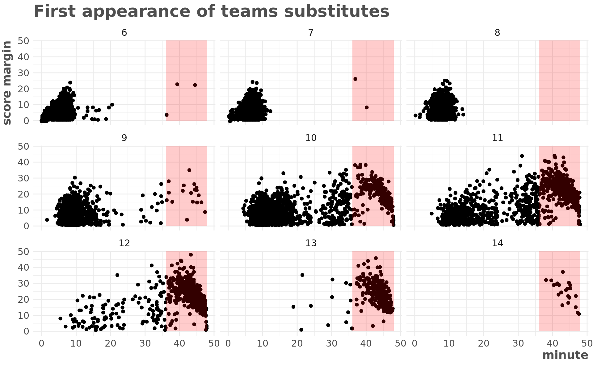
Based on this chart, I think we can be fairly safe if we say that garbage time starts when the 12th player enters in the 4th quarter.
Let’s apply that definition to all of the games to see when garbage time starts or what the final margin was if it didn’t happen.
gt_start <- player_starts %>%
    group_by(idGame) %>%
    filter(n_player == 12,
           max(minuteGame) <= 48, # no ot
           minuteGame >= 36) %>%
    filter(minuteGame == min(minuteGame)) %>%
    ungroup() %>%
    distinct(minuteGame, idGame, marginScore) %>%
    select(idGame, gt_start = minuteGame, gt_margin = marginScore)

fill_margin <- function(dat){

    dat %>%
        fill(marginScore) %>%
        replace_na(list(marginScore = 0))

}

pbp_gt <- games_pbp %>%
    group_by(idGame) %>%
    filter(max(minuteGame) <= 48) %>%
    ungroup() %>%
    split(.$idGame) %>%
    map_dfr(fill_margin) %>%
    left_join(gt_start, by = "idGame") %>%
    mutate(
        gt = case_when(
            is.na(gt_start) ~ 0L,
            minuteGame >= gt_start ~ 1L,
            TRUE ~ 0L
        )
    )
Now we have play-by-play for each game and whether garbage time had kicked in.
How many games went to garbage time?
pbp_gt %>%
    arrange(desc(gt)) %>%
    distinct(idGame, .keep_all = TRUE) %>%
    summarise(mean_gt = scales::percent(mean(gt)))
## # A tibble: 1 x 1
## mean_gt
## <chr>
## 1 34%That sounds about right to me.
What is was the score margin and time when garbage time began?
pbp_gt %>%
    filter(gt == 1) %>%
    group_by(idGame) %>%
    arrange(minuteGame, desc(marginScore)) %>%
    distinct(idGame, .keep_all = TRUE) %>%
    select(idGame, marginScore, minuteGame) %>%
    ggplot(aes(minuteGame, abs(marginScore))) +
geom_point() 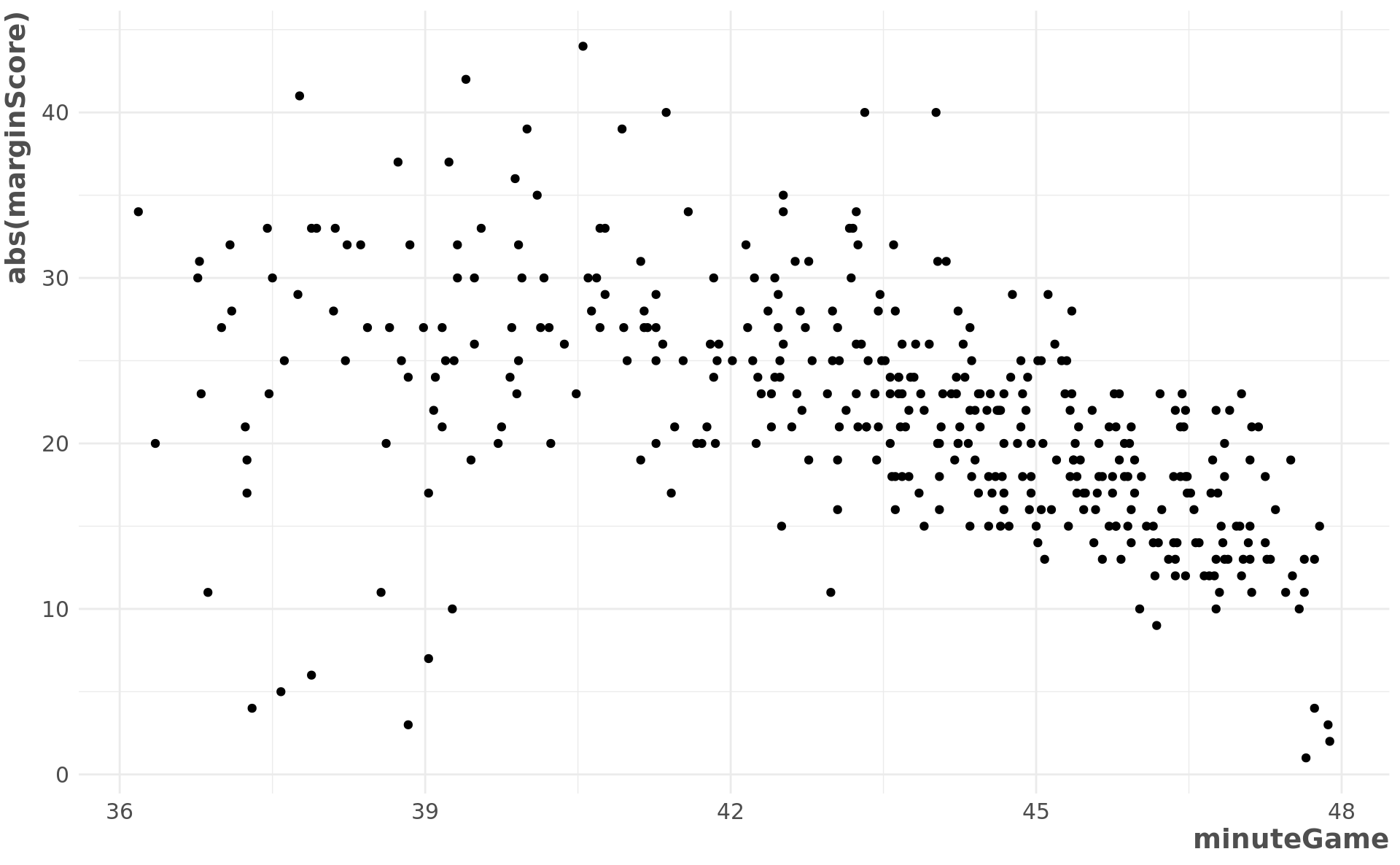
Modeling
There’s a few different ways to define this problem that will influence our modeling choices moving forward.
- What is the relationship between game time and score margin when garbage time starts? (regression)
- What is the probability of a game having entered garbage time at a given time and score margin? (survival analysis)
- When is a game decided (how likely is that the team ahead at a given point and score margin will finish the game as the winner)? (logisitc regression)
The first two represent how coaches make the decision to put in their deepest bench players while the last question has to do with the probability of the outcome.
Regression model
Here we’ll examine the relationship between score margin and game time. I use the rethinking package that provides an interface to Stan for estimating Bayesian posterior distributions.
reg_df <- pbp_gt %>%
    group_by(idGame) %>%
    filter(gt == 1) %>%
    arrange(minuteGame) %>%
    distinct(idGame, .keep_all = TRUE) %>%
    select(idGame, minuteGame, marginScore, gt) %>%
    mutate(marginScore = abs(marginScore))

reg_list <- list(
    t = reg_df$minuteGame - 36,
    m = reg_df$marginScore
)

set.seed(2020)

reg_mod <- ulam(
    alist(
        m ~ normal(mu, sigma),
        mu <-  -exp(b1 * t) + a,
        sigma ~ exponential(1),
        b1 ~ normal(0.25, 0.01),
        a ~ normal(35, 7)
    ),
    data = reg_list,
    chains = 4,
    cores = parallel::detectCores()
)


pred_df <- tibble(t = seq(0, 12, by = 0.1))

reg_preds <- link(reg_mod, pred_df)

pred_mean <- apply(reg_preds, 2, mean)
pred_ci <- apply(reg_preds, 2, PI)

margin_pred <- pred_df %>%
    mutate(
        mean = pred_mean,
        low = pred_ci[1, ],
        high = pred_ci[2, ]
    )

margin_pred %>%
    ggplot(aes(t, mean)) +
        geom_line() +
        geom_point(data = reg_df, aes(minuteGame - 36, marginScore)) +
        geom_ribbon(aes(ymin = low, ymax = high), alpha = 0.2) +
        scale_x_continuous(limits = c(0, 12)) +
        labs(
            x = "game minute",
            y = "score margin",
            title = "Predicted score margin of entering garbage time"
        )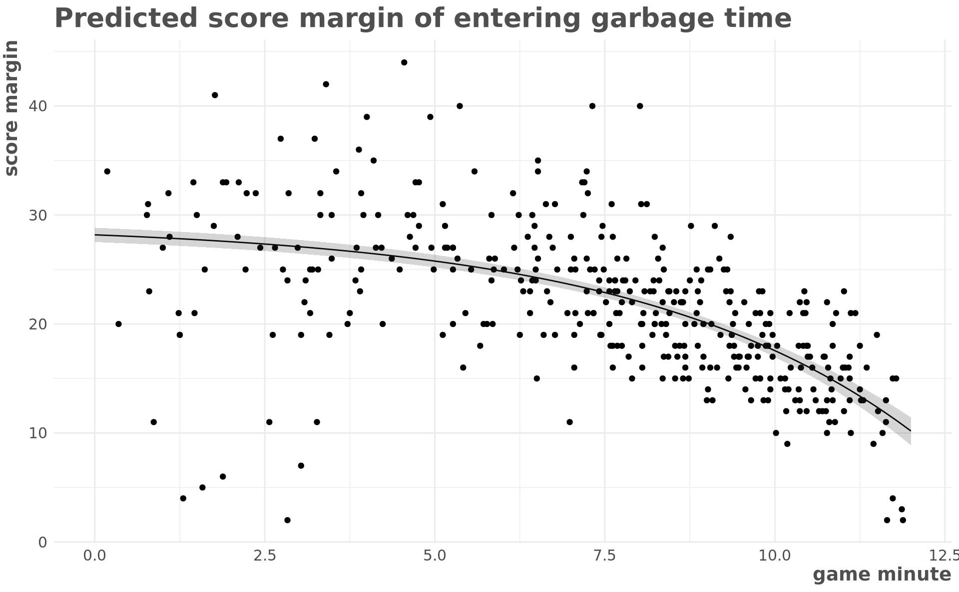
This model gives us the estimate of the score margin that we expect garbage time to kick in at each point in time. It seems to fit the data well, but it may not be the most informative way to formulate the question.
Survival analysis
Survival analysis is fundamentally about time to event. Here we’ll use a Cox Proportional Hazard model which takes the probability of a team not entering garbage time a given point in time, and factors in a parameter for the score margin.
surv_df <- pbp_gt %>%
    mutate(minuteGame = round(minuteGame, 1)) %>%
    arrange(minuteGame, desc(gt)) %>%
    distinct(idGame, minuteGame, .keep_all = TRUE) %>%
    complete(idGame, minuteGame)  %>%
    fill(gt, marginScore) %>%
    replace_na(list(gt = 0, marginScore = 0)) %>%
    group_by(idGame, gt) %>%
    mutate(
        keep = case_when(
            gt == 0 & minuteGame == 48 ~ 1,
            gt == 1 & minuteGame == min(minuteGame) ~ 1,
            TRUE ~ 0
        )
    ) %>%
    filter(keep == 1) %>%
    ungroup() %>%
    select(idGame, minuteGame, marginScore, gt)


cox_fit <- coxph(Surv(minuteGame, gt) ~ log(marginScore), data = surv_df)

cox_sim <- crossing(
  marginScore = seq(0, 30, by = 5)
)

cox_pred <- survfit(cox_fit, newdata = cox_sim)

cox_df <- as_tibble(cox_pred$cumhaz)

colnames(cox_df) <- cox_sim$marginScore

surv_preds <- cox_df %>%
    mutate(minuteGame = cox_pred$time) %>%
    gather(margin, haz_prob, -minuteGame, convert = TRUE)

surv_preds %>%
    mutate(margin = fct_rev(factor(margin))) %>%
    ggplot(aes(minuteGame, haz_prob, color = margin)) +
        geom_line(size = 1.5) +
        scale_y_continuous(limits = c(0, NA), labels = scales::percent) +
        labs(
            title = "Cumulative hazard curves for garbage time",
            y = "cumulative hazard of entering garbage time",
            x = "minute in game",
            color = "score margin",
            caption = "hazards are cumulative and can sum to greater than one"
        )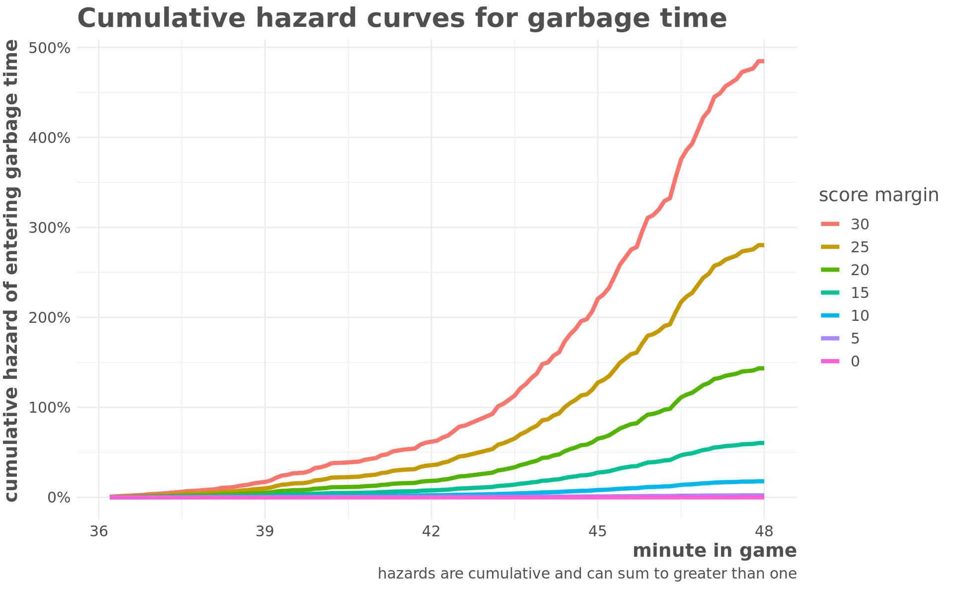
Since the hazards are cumulative, they can have a greater than 100% probability. One limitation of this model is that is that the score margins are based on an average, so it seems to be overestimating the probability of entering garbage time for low margin games. For example, a game that has a 10-point margin with 3 minutes to go would be considered a close scoring game, but this model estimates it has a 25% probability of entering garbage time.
When is a game decided?
The other way to look at garbage time is to examine at what point the outcome is already decided. Below I’ll fit a logistic regression that calculates the probability that the team ahead at a given point in time ends up winning. We’ll also factor in whether the team is home or away as home teams have a higher chance of winning the game from the start, all other things being equal.
scores_df <- games_pbp %>%
    mutate(minuteGame = round(minuteGame, 1)) %>%
    complete(idGame, minuteGame = seq(0, 48, by = 0.1)) %>%
    group_by(idGame) %>%
    fill(marginScore) %>%
    replace_na(list(marginScore = 0)) %>%
    arrange(minuteGame, desc(marginScore)) %>%
    distinct(idGame, minuteGame, .keep_all = TRUE) %>%
    select(idGame, minuteGame, marginScore) %>%
    filter(minuteGame <= 48) %>%
    ungroup()

final_scores <- scores_df %>%
    group_by(idGame) %>%
    filter(minuteGame == max(minuteGame)) %>%
    distinct(idGame, .keep_all = TRUE) %>%
    select(idGame, final_score = marginScore)

scores_w_final <- scores_df %>%
    inner_join(final_scores, by = "idGame") %>%
    transmute(
        home_margin = marginScore,
        away_margin = -marginScore,
        home_final = final_score,
        away_final = -final_score,
        idGame,
        minuteGame
    ) %>%
    gather(metric, margin, -idGame, -minuteGame) %>%
    separate(metric, c("team", "type")) %>%
    spread(type, margin) %>%
    mutate(win = final > 0) %>%
    filter(margin >= 0)

win_mod <- glm(
    win ~ exp(margin) + margin:minuteGame + minuteGame:team + team,
    data = scores_w_final,
    family = "binomial"
)

win_preds <- crossing(
    minuteGame = seq(0, 48, by = 0.1),
    margin = seq(0, 30, by = 5),
    team = c("home", "away")
) %>%
    broom::augment(win_mod, newdata = ., type.predict = "response") %>%
    rename(win_prob = .fitted, win_se = .se.fit)

win_preds %>%
    mutate(margin = fct_rev(factor(margin))) %>%
    ggplot(aes(minuteGame, win_prob, color = factor(margin), linetype = team)) +
        geom_line(size = 1.5) +
        scale_y_continuous(labels = scales::percent, limits = c(0, 1)) +
        labs(
            title = "Probability that games the winning team at time\nwill win game",
            y = "probability of winning",
            x = "game minute",
            color = "current margin",
            linetype = ""
        )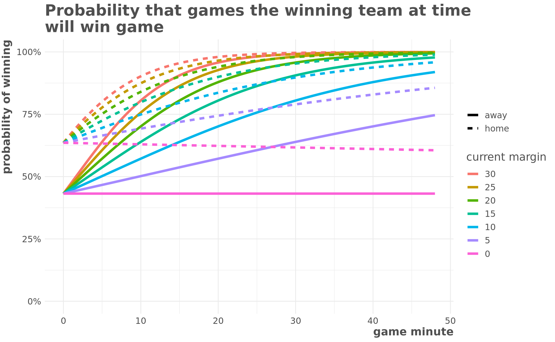
There are a few interesting things happening here. You can see the home team’s advantage diminishing over time. Games with a 30 point margin are basically decided at half time, and overcoming a 20 point deficit in the 4th quarter is quite rare.
However, there are a few limitations of this model. The home and away margin should converge at the end of regulation and all other margins should be at 1 at minute 48. These are limitations of how we defined our model.
Putting it together
margins <- seq(0, 30, by = 5)

time_preds <- margin_pred %>%
    gather(metric, margin, -t) %>%
    mutate(margin = round(margin, 0)) %>%
    filter(margin %in% margins) %>%
    group_by(margin) %>%
    summarise(
        low_time = min(t),
        mid_time = median(t),
        high_time = max(t)
    ) %>%
    mutate_at(vars(low_time:high_time), function(x) x + 36)

win_preds %>%
  left_join(surv_preds, by = c("margin", "minuteGame")) %>%
  left_join(time_preds, by = "margin") %>%
  select(-win_se) %>%
  gather(metric, val, win_prob:haz_prob) %>%
  mutate(team = if_else(metric == "haz_prob", "away", team)) %>%
  group_by(metric, margin) %>%
  arrange(minuteGame) %>%
  fill(val) %>%
  replace_na(list(val = 0)) %>%
  ggplot(aes(minuteGame, val,linetype = team, color = metric)) +
    geom_line(size = 1.5) +
    geom_hline(yintercept = 1, linetype = 2, alpha = 0.5, color = jtc_primary[[1]]) +
    geom_rect(aes(ymin = 0, ymax = Inf, xmin = low_time, xmax = high_time),
              inherit.aes = FALSE, alpha = 0.05, fill = jtc_greys[[3]]) +
    facet_wrap(~ margin) +
    scale_x_continuous(limits = c(0, 48), breaks = seq(0, 48, by = 12)) +
    scale_y_continuous(
      limits = c(0, 1.25), labels = scales::percent,
      breaks = seq(0, 1, by = 0.25)
    ) +
    scale_color_manual(
        labels = c("cumulative hazard", "win probability"),
        values = jtc_primary[c(2,3)]
    ) +
    labs(
      linetype = "",
      color = "",
      y = "",
      x = "game minute",
      title = "Coaches put in deep bench reserves after\ngame is decided",
      subtitle = "Model predictions at different score margins",
      caption = "Vertical grey bars show estimates of entering garbage time from regression model"
) 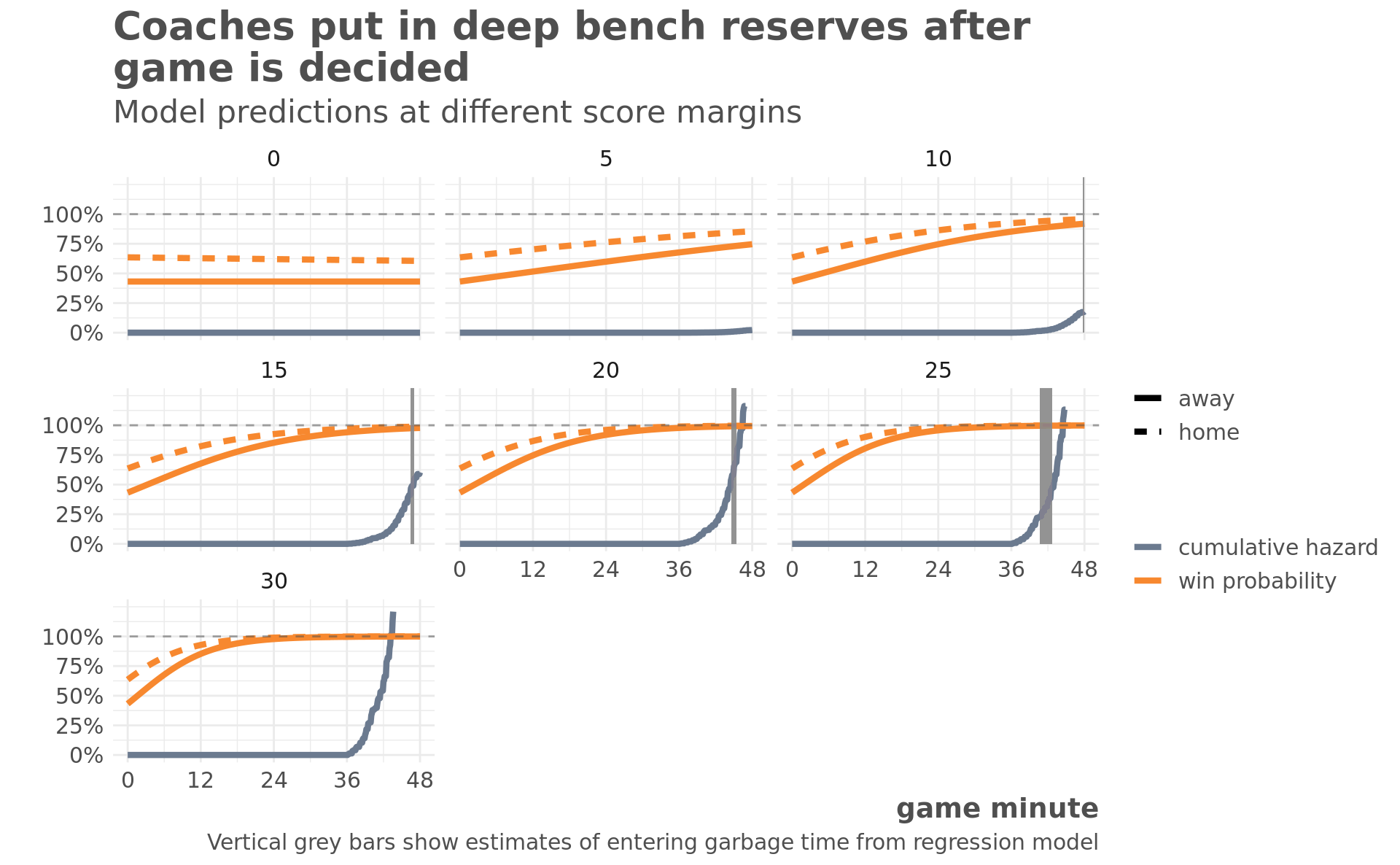
This chart is showing all three models together broken down by a range of margins. The blue lines show the cumulative hazard curves of survival model, the orange lines show the probability of winning at each point in the game for each margin, and the vertical grey bars show the estimate of the most likely time of entering garbage time1.
Unsurprisingly, coaches seem to have a very low risk tolerance to putting in their deep bench players when the game has been decided beyond any doubt.
Other questions
There are a number of other questions that would be interesting to explore in this problem.
- What are other ways to define garbage time start (than a player’s first action)?
- How do coaches differ in whether or not they go into garbage time mode?
- How does the time of season factor in?
- Has the boundary for garbage time changed over time?
- How close does the score have to get for a coach to put their starters back in?
- How to factor in games going to overtime?
Conclusion
I set out here to examine the question of when garbage time does and should start. As I went along, I became interested in how the different problem definitions led to different modeling choices. Each of the different models we chose gives insight into the question we asked it; however, each also has tradeoffs. It’s important to understand how different framings of a similar questions lead to modeling decisions and therefore to insight we gain from an analysis.
What are other ways that we could address the question of when garbage time does and should start? How could we improve the models presented here. Feel free to share any feedback you have.
The regression model predicts that margins less than 10 will ‘enter’ garbage time after the 48th minute and scores pver 30 enter garbage time before the 4th quarter, inconsistent with our definition.↩
