
Is it more likely to rain on Tuesdays in Philadelphia?
Trash day in our neighborhood is on Wednesday, which means we have to put our trash out on Tuesday night. My wife and I always joke that it seems to rain more on Tuesdays than any other day. This may not seem like a thing to even notice, except that in our South Philly row home, we have to lug soaking wet trash cans and recycling bins from our backyard through our kitchen and living to put them out on the sidewalk each week.
Does our observation hold up? I downloaded data on Philadelphia weather1 from 2009 (when we moved in to our current home) to present to see.
library(tidyverse)
library(lubridate)
library(here)
library(broom)
library(huxtable)

weather <- "https://jtcies.com/data/phl_weather_20090925-20180924.csv" %>%
  read_csv()
## Warning: 1697 parsing failures.
## row col expected actual file
## 1285 TAVG 1/0/T/F/TRUE/FALSE 51 'https://jtcies.com/data/phl_weather_20090925-20180924.csv'
## 1286 TAVG 1/0/T/F/TRUE/FALSE 42 'https://jtcies.com/data/phl_weather_20090925-20180924.csv'
## 1287 TAVG 1/0/T/F/TRUE/FALSE 40 'https://jtcies.com/data/phl_weather_20090925-20180924.csv'
## 1288 TAVG 1/0/T/F/TRUE/FALSE 41 'https://jtcies.com/data/phl_weather_20090925-20180924.csv'
## 1289 TAVG 1/0/T/F/TRUE/FALSE 48 'https://jtcies.com/data/phl_weather_20090925-20180924.csv'
## .... .... .................. ...... ...........................................................
## See problems(...) for more details.glimpse(weather)## Observations: 3,284
## Variables: 33
## $ STATION <chr> "USW00013739", "USW00013739", "USW00013739", "USW00013739",…
## $ NAME <chr> "PHILADELPHIA INTERNATIONAL AIRPORT, PA US", "PHILADELPHIA …
## $ LATITUDE <dbl> 39.87327, 39.87327, 39.87327, 39.87327, 39.87327, 39.87327,…
## $ LONGITUDE <dbl> -75.22678, -75.22678, -75.22678, -75.22678, -75.22678, -75.…
## $ ELEVATION <dbl> 3, 3, 3, 3, 3, 3, 3, 3, 3, 3, 3, 3, 3, 3, 3, 3, 3, 3, 3, 3,…
## $ DATE <date> 2009-09-25, 2009-09-26, 2009-09-27, 2009-09-28, 2009-09-29…
## $ AWND <dbl> 9.84, 7.83, 8.28, 10.29, 16.11, 9.62, 8.05, 6.93, 2.01, 7.1…
## $ PRCP <dbl> 0.00, 0.24, 0.77, 0.27, 0.00, 0.00, 0.00, 0.03, 0.01, 0.00,…
## $ PSUN <lgl> NA, NA, NA, NA, NA, NA, NA, NA, NA, NA, NA, NA, NA, NA, NA,…
## $ SNOW <dbl> 0, 0, 0, 0, 0, 0, 0, 0, 0, 0, 0, 0, 0, 0, 0, 0, 0, 0, 0, 0,…
## $ SNWD <dbl> 0, 0, 0, 0, 0, 0, 0, 0, 0, 0, 0, 0, 0, 0, 0, 0, 0, 0, 0, 0,…
## $ TAVG <lgl> NA, NA, NA, NA, NA, NA, NA, NA, NA, NA, NA, NA, NA, NA, NA,…
## $ TMAX <dbl> 75, 69, 75, 79, 70, 64, 59, 68, 76, 74, 68, 68, 72, 67, 80,…
## $ TMIN <dbl> 56, 54, 59, 57, 53, 53, 48, 47, 60, 55, 50, 48, 56, 48, 59,…
## $ TSUN <lgl> NA, NA, NA, NA, NA, NA, NA, NA, NA, NA, NA, NA, NA, NA, NA,…
## $ WT01 <dbl> NA, NA, 1, NA, NA, NA, NA, 1, 1, 1, NA, NA, 1, NA, NA, NA, …
## $ WT02 <dbl> NA, NA, NA, NA, NA, NA, NA, NA, NA, NA, NA, NA, NA, NA, NA,…
## $ WT03 <dbl> NA, NA, NA, NA, NA, NA, NA, NA, NA, NA, NA, NA, NA, NA, NA,…
## $ WT04 <dbl> NA, NA, NA, NA, NA, NA, NA, NA, NA, NA, NA, NA, NA, NA, NA,…
## $ WT05 <dbl> NA, 1, 1, 1, NA, 1, NA, 1, NA, NA, NA, NA, 1, NA, 1, NA, NA…
## $ WT06 <dbl> NA, NA, NA, NA, NA, NA, NA, NA, NA, NA, NA, NA, NA, NA, NA,…
## $ WT07 <dbl> NA, NA, NA, NA, NA, NA, NA, NA, NA, NA, NA, NA, NA, NA, NA,…
## $ WT08 <dbl> NA, NA, NA, NA, NA, NA, NA, NA, NA, NA, NA, NA, NA, NA, NA,…
## $ WT09 <dbl> NA, NA, NA, NA, NA, NA, NA, NA, NA, NA, NA, NA, NA, NA, NA,…
## $ WT11 <dbl> NA, NA, NA, 1, NA, NA, NA, NA, NA, NA, NA, NA, NA, NA, NA, …
## $ WT13 <dbl> NA, NA, 1, NA, NA, NA, NA, NA, 1, NA, NA, NA, 1, NA, NA, NA…
## $ WT14 <dbl> NA, NA, 1, NA, NA, NA, NA, NA, NA, NA, NA, NA, NA, NA, NA, …
## $ WT15 <dbl> NA, NA, NA, NA, NA, NA, NA, NA, NA, NA, NA, NA, NA, NA, NA,…
## $ WT16 <dbl> NA, 1, 1, 1, NA, 1, NA, 1, 1, NA, NA, 1, 1, 1, 1, 1, NA, NA…
## $ WT17 <lgl> NA, NA, NA, NA, NA, NA, NA, NA, NA, NA, NA, NA, NA, NA, NA,…
## $ WT18 <dbl> NA, NA, NA, NA, NA, NA, NA, NA, NA, NA, NA, NA, NA, NA, NA,…
## $ WT21 <dbl> NA, NA, NA, NA, NA, NA, NA, NA, 1, NA, NA, NA, NA, NA, NA, …
## $ WT22 <dbl> NA, NA, NA, NA, NA, NA, NA, NA, NA, NA, NA, NA, NA, NA, NA,…I requested a bunch of variables when getting the data initially because I thought some might might be useful in the future. The only two we care about here are DATE and PRCP which is daily rainfall total in inches. Let’s check to make sure we got the dates we requested.
range(weather$DATE)## [1] "2009-09-25" "2018-09-21"Looks good. Using the wday function from the lubridate package, we can easily get the day of the week for any date.
weather <- weather %>%
  mutate(
    day_of_week = wday(DATE, label = TRUE)
  )

count(weather, day_of_week) %>%
  as_hux() %>%
  add_colnames() %>%
theme_article()| day_of_week | n |
|---|---|
| day_of_week | n |
| Sun | 469 |
| Mon | 469 |
| Tue | 469 |
| Wed | 469 |
| Thu | 469 |
| Fri | 470 |
| Sat | 469 |
Perfect.
Total rainfall
Let’s get a picture of the distribution of rain.
ggplot(weather, aes(x = PRCP)) +
  geom_histogram(binwidth = 0.1)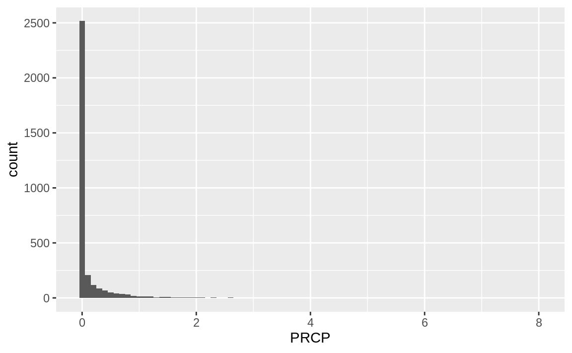
Rainfall totals are highly skewed becuse there is no rain most of the of time. We can log transfrom it to get a sense of how rainfall total differs on days of the week.
ggplot(weather, aes(x = day_of_week, y = log(PRCP + 0.0001))) +
  geom_boxplot()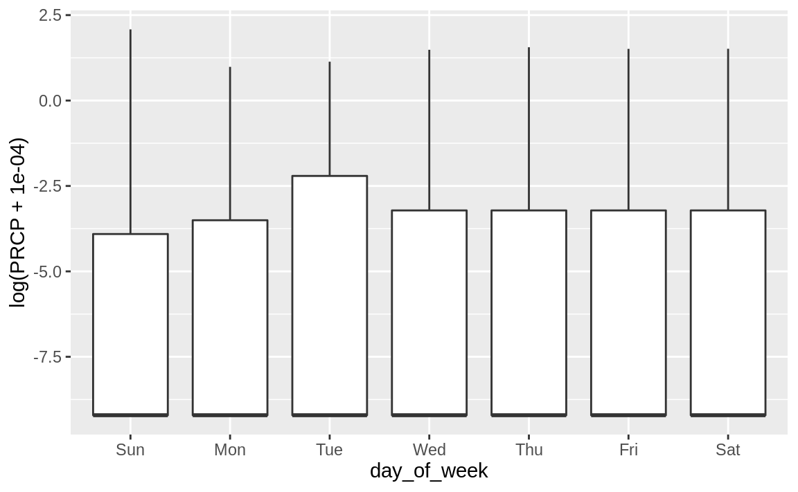
Ok, so it actually looks like Tuesdays get more rain than other days. I wasn’t really expecting this but we’ll roll with it.
Did it rain at all?
However, this doesn’t really answer the question we’re interested in. We don’t care too much about the amount of rain that fell. Really we want to know if it is more likley to rain at all on Tuesdays. To do this we’ll create a binary variable that is 1 if it rained more than 0 inches, and 0 otherwise.
weather <- weather %>%
  mutate(
    rain = if_else(PRCP > 0, 1L, 0L)
  )

weather %>%
  group_by(day_of_week) %>%
  summarise(avg_days_rain = mean(rain)) %>%
  as_hux() %>%
  add_colnames() %>%
theme_article()| day_of_week | avg_days_rain |
|---|---|
| day_of_week | avg_days_rain |
| Sun | 0.286 |
| Mon | 0.32 |
| Tue | 0.386 |
| Wed | 0.326 |
| Thu | 0.341 |
| Fri | 0.306 |
| Sat | 0.318 |
Wait … what? It actually does rain more on Tuesdays. By quite a bit. Almost 40% of the time compared to less than 30% of Sundays.
We can create a logistic regression model to help us figure out whether this result is likley to be just due to variation in the data or whether there is some underlying pattern here.
fit <- weather %>%
  mutate(day_of_week = as.character(day_of_week)) %>%
  glm(
    rain ~ day_of_week,
    family = "binomial",
    data = .
  )

fit_tidy <- fit %>%
  broom::tidy()

fit_tidy %>%
  select(term, estimate, p.value) %>%
  as_hux() %>%
  add_colnames() %>%
theme_article()| term | estimate | p.value |
|---|---|---|
| term | estimate | p.value |
| (Intercept) | -0.817 | 3.19e-16 |
| day_of_weekMon | 0.0625 | 0.657 |
| day_of_weekSat | 0.0527 | 0.708 |
| day_of_weekSun | -0.0992 | 0.488 |
| day_of_weekThu | 0.159 | 0.255 |
| day_of_weekTue | 0.353 | 0.0105 |
| day_of_weekWed | 0.0918 | 0.513 |
Let’s plot these coefficients.
fit_tidy %>%
  ggplot(aes(x = reorder(term, desc(estimate)),
             y = estimate,
             ymin = estimate - (1.96 * std.error),
             ymax = estimate + (1.96 * std.error))) +
    geom_pointrange(color = "#6b7a8f") +
    coord_flip() +
    labs(
      title = "It is significantly more likley to rain on Tuesdays",
      subtitle = "lines show 95% confidence intervals",
      x = "Term (day of the week)",
      y = "coefficients"
) 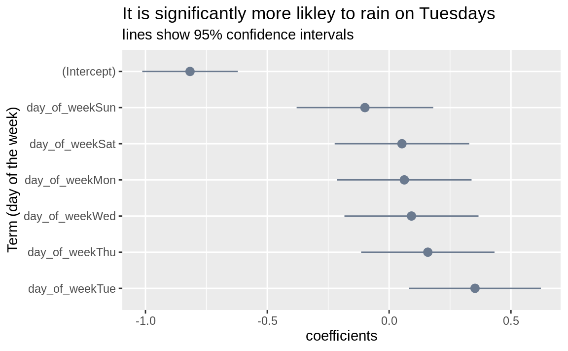
Of the coefficients for the days of the week, Tuesday is the only one whose range does not include zero. This means that, based on our model, it is significantly likely that it’s more likley to rain on Tuesdays than on other days.
When we add the coefficent for a day to the incercept (which is the same for each day), we get the log odds that it will rain on that day, based solely on the day of the week. Friday is the reference day (because it’s the first alphabetically), so the intercept represents the log odds of rain on Fridays. Once we have the log odds, we can convert it back to a standard probability.
To find probability of rain on Tuesday:
intercept <- as.numeric(fit_tidy$estimate[fit_tidy$term == "(Intercept)"])
tues_coef <- as.numeric(fit_tidy$estimate[fit_tidy$term == "day_of_weekTue"])

tues_logit <- intercept + tues_coef

tues_odds <- exp(tues_logit)

tues_prob <- tues_odds / (1 + tues_odds)

tues_prob
## [1] 0.3859275We knew this from the table above, but would be useful if we added more variables to our model.
So what’s going on here?
I wasn’t expecting find this. In fact, I assumed it was just my annoyance that it was once again trash night that made me more notice the rain. However, the observed data indicates that it is more likley to rain on Tuesday. The question is whether there is some underlying weather pattern designed to increase my annoyance on trash night?
Maybe. But most likley this is just a chance result. In reality, the true probability that it rains more on Tuesdays is really not higher than the chance that it rains on any other day. The fact that it has rained more on Tuesdays is just a coincidence. While statistics is meant help us parse observed data to discover underling truths, it can only speak to us in terms of probabilities and likelihoods.
Perhaps there is some lesson here about being careful about inferences made from statistics, especially when they seem suspect. Or maybe I should just move to a neighborhood where you put your trash out on Fridays.
