
Quantifying uncertainty around the short MLB season
This year’s going to be a weird year for baseball. Many have commented how the shortened season could lead to some weird final results, with highest ranked teams finishing lower than expected or some pretty bad teams ending with a decent record. This is because the outcome of any one game of baseball contains relatively little information about which team is actually better in the long run.
The question then, is what’s the amount of uncertainty we have about how teams will finish compared to a normal season? Seems like a problem for Bayesian statistics …
Setup
We’ll build a simple model to predict a team’s wins using their preseason odds of winning the World Series. We’ll use 2019 data to build the model, and then see how how the results change using the 2020 odds comparing a normal season to a short one.
First we’ll scrape the data on 2019 results and odds for 2019 and 2020.
library(tidyverse)
library(rvest)
library(jtcr)
library(ggrepel)
library(scales)
library(rethinking)

theme_set(theme_jtc())

## get 2019 results
results_2019_url <- "https://en.wikipedia.org/wiki/2019_Major_League_Baseball_season"

names_2019 <- c("team", "wins", "losses", "pct", "games_back",
                "home", "road")

rename_table <- function(x) {
    names(x) <- names_2019
    x
}

leagues <- c("ALE", "ALC", "ALW", "NLE", "NLC", "NLW")

results_2019 <- read_html(results_2019_url) %>%
    html_nodes(".wikitable .wikitable") %>%
    purrr::map(html_table) %>%
    map_dfr(rename_table, .id = "league") %>%
    na_if(list(games_back = "—")) %>%
    mutate(
        team = str_remove(team, "\\([0-9]\\)"),
        league = leagues[as.numeric(league)]
    ) %>%
    arrange(team)

## get 2019 preseason odds

odds_2019_url <- "https://www.betcris.com/articles/baseball/mlb/mlb-futures-2019-world-series-odds-92616"

odds_2019 <- read_html(odds_2019_url) %>%
    html_nodes("h2~ p , p p") %>%
    html_text() %>%
    .[1:30] %>%
    enframe() %>%
    select(-name) %>%
    separate(value, into = c("team", "odds"), sep = " \\+") %>%
    mutate(odds = parse_number(odds),
           year = 2019)

## get 2020 preseason odds

odds_2020_url <- "https://www.betcris.com/en/articles/baseball/mlb/mlb-baseball-world-series-odds-97157"

odds_2020 <- read_html(odds_2020_url) %>%
    html_nodes("td") %>%
    html_text() %>%
    .[2:31] %>%
    enframe() %>%
    select(-name) %>%
    separate(value, into = c("team", "odds"), sep = " \\+") %>%
    mutate(odds = parse_number(odds),
           year = 2020,
           team = str_replace(team, "Saint", "St."))

odds <- bind_rows(odds_2019, odds_2020) %>%
    arrange(team)
First let’s take a look at the distributions. Below is a plot that shows win percentage of a team that is expected to win 50% of their games based on 100,000 simulations of seasons either normal lengths (162 games) or shortened (60 games).
short <- rbinom(1e5, 60, prob = 0.5) / 60
long <- rbinom(1e5, 162, prob = 0.5) / 162

tibble(short, long) %>%
    gather() %>%
    ggplot(aes(value, fill = key, color = key)) +
        geom_density(bw = 0.02, alpha = 0.5) +
        scale_x_continuous(labels = percent) +
        labs(title = "Simulated win percentage for a team with 50% win probability",
             subtitle = "based on 100,000 simulations",
             x = "win percentage",
             y = "density")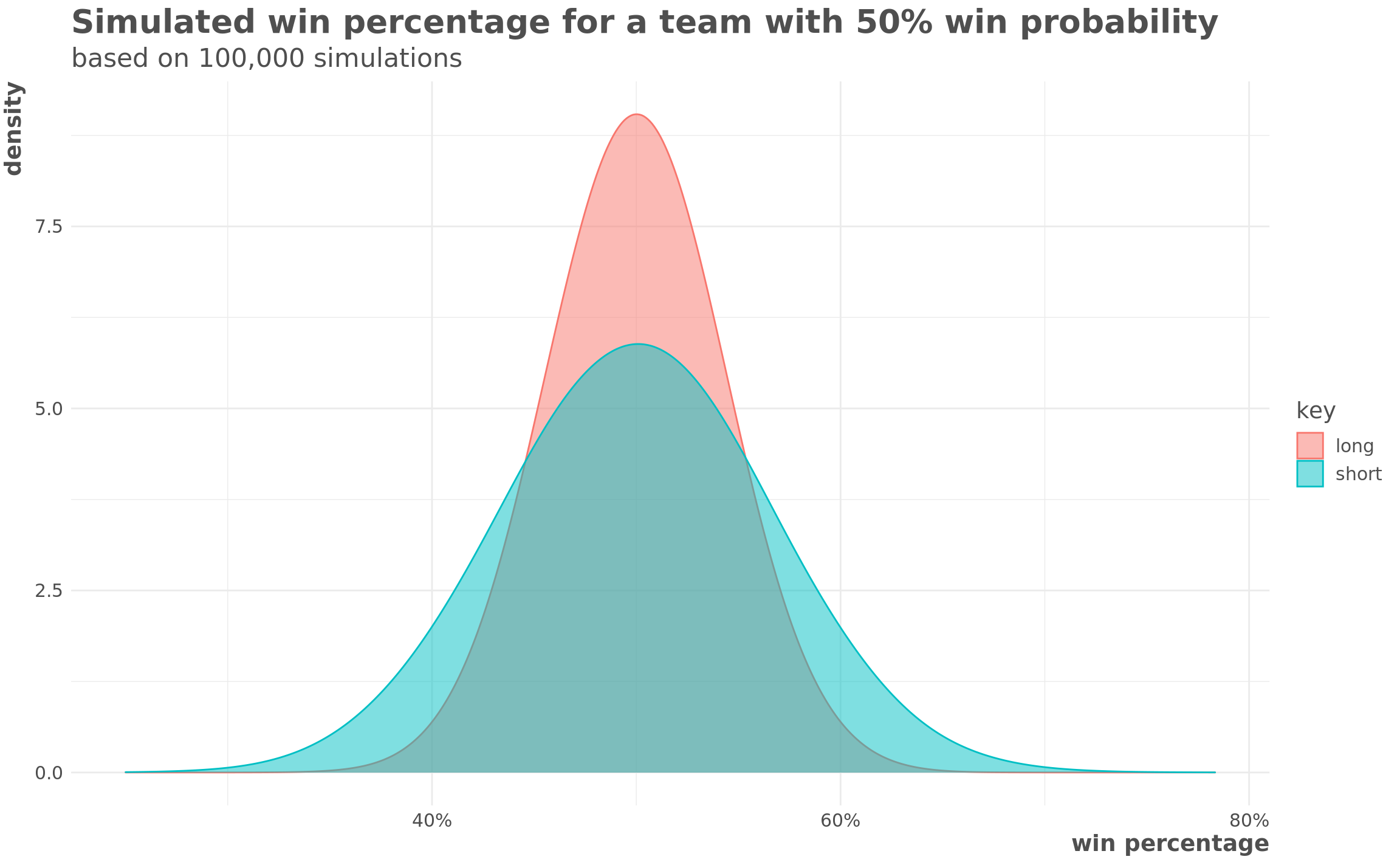
short_40 <- pbinom(60 * 0.4, 60, prob = 0.5)
long_40 <- pbinom(162 * 0.4, 162, prob = 0.5)
In our imaginary world where this team has a 50% probability of winning every game, in short season that team would end up winning 40% or fewer of its games 7.8% of the time, while in a normal season that would only happen 0.5%of the time.
Modeling
We’ll build a model to predict win percentage based on preseason odds of winning the World Series. Below are those odds:
odds %>%
    mutate(team = fct_reorder(team, -odds)) %>%
    ggplot(aes(team, odds, color = factor(year))) +
        geom_point(size = 2) +
        coord_flip() +
        scale_y_continuous(labels = function(x) paste0("+", comma(x)),
                           trans = "log10") +
        labs(title = "Comparing World Series champion odds between years",
             y = "odds of winning World Series (log scale)",
             x = "",
             color = "season",
             caption = "odds from betcris.com")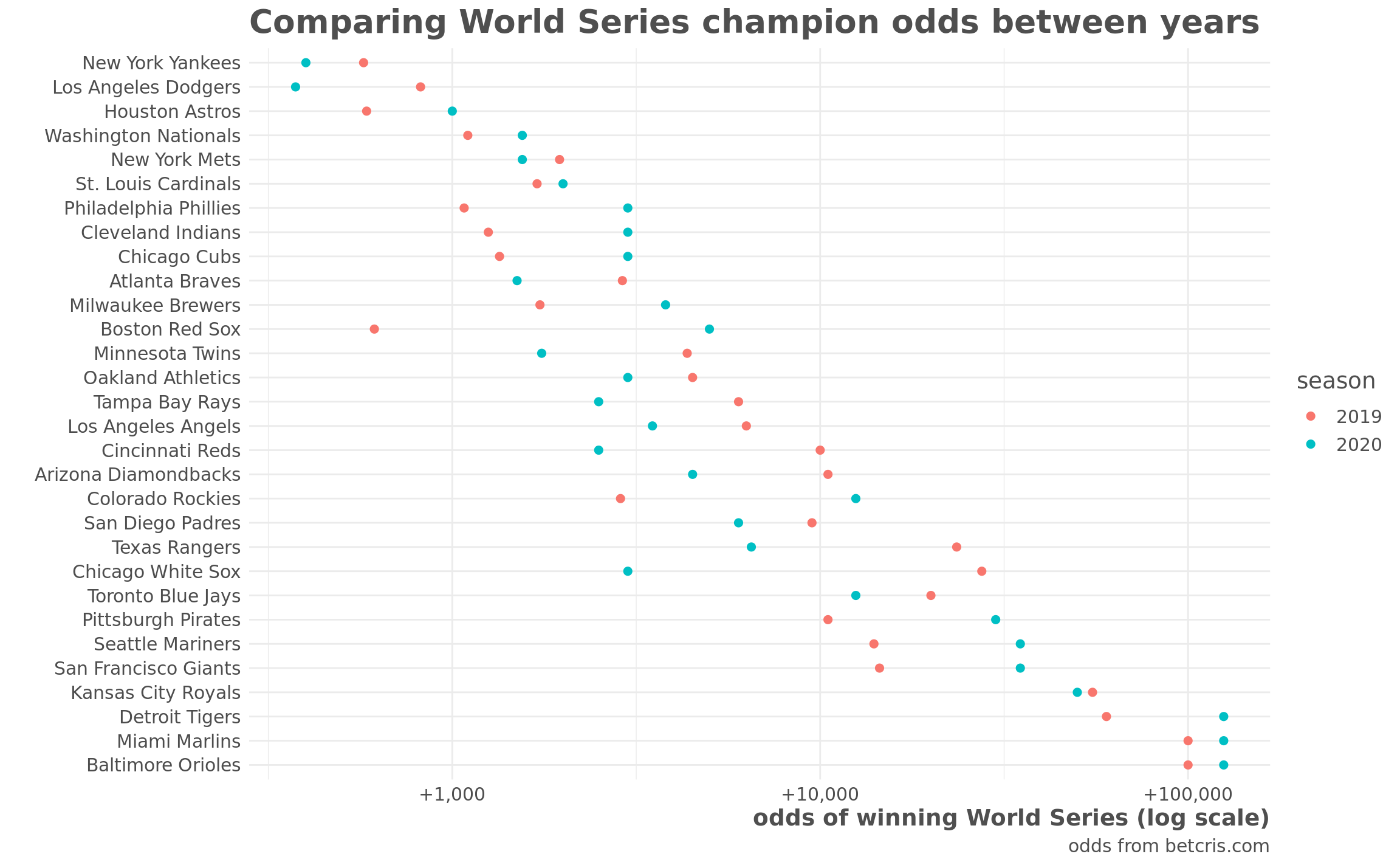
And below is how the 2019 odds compared to each time’s final regular season win percentage:
odds %>%
    filter(year == 2019) %>%
    inner_join(results_2019, by = "team") %>%
    ggplot(aes(odds, pct)) +
        geom_point() +
        geom_text_repel(aes(label = team)) +
        scale_x_log10(labels = scales::comma) +
        scale_y_continuous(labels = scales::percent) +
        labs(x = "preseason World Series odds",
             title = "Preseason World Series odds and final win percentage",
             subtitle = "2019 season",
             y = "win percentage")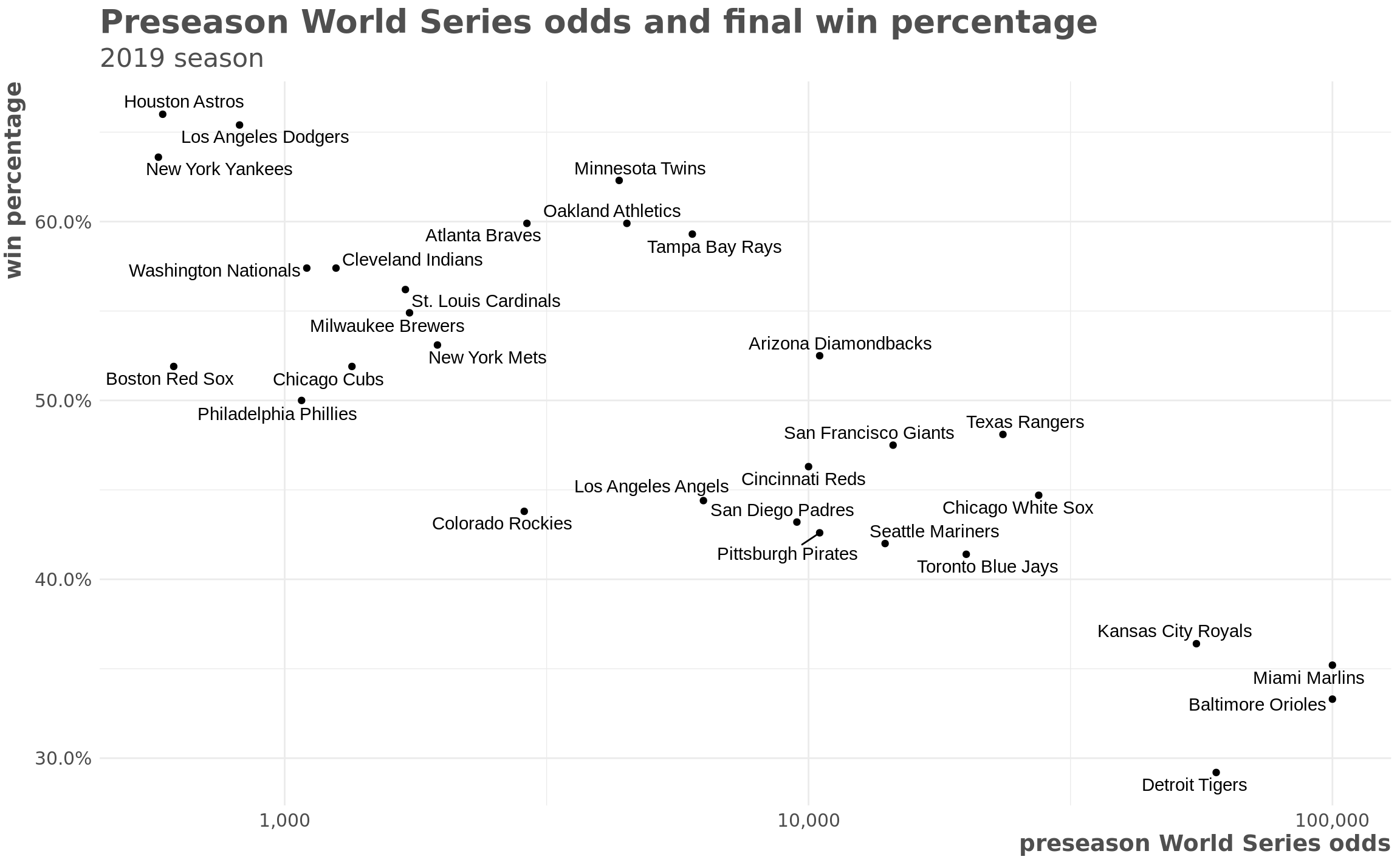
Prior predictive checks
Our model is a logistic regression that looks like:
\[ W_i \sim {\sf Binom}(n, p_i) \\ logit(p_i) = \alpha + \beta * O_i \\ \alpha \sim \mathcal{N}(0, 1) \\ \beta \sim \mathcal{N}(0, 0.5) \]
where \(W\) is number of wins in a season, \(n\) is the number of games in a season, and \(O\) is the log odds of a team winning the World Series before the season starts.
First, we check our priors to make sure they produce reasonable results.
b_prior <- rnorm(20, 0, 0.5)
a_prior <- rnorm(20, 0, 1)
odds_sample <- 0:12

wins_prior_pred <- crossing(a_prior,
                            b_prior,
                            odds = odds_sample) %>%
    group_by(odds) %>%
    mutate(p = inv_logit(a_prior + b_prior * odds),
           group = row_number()) %>%
    ungroup()

wins_prior_pred %>%
    ggplot(aes(odds, p, group = group)) +
        geom_line(alpha = 0.2)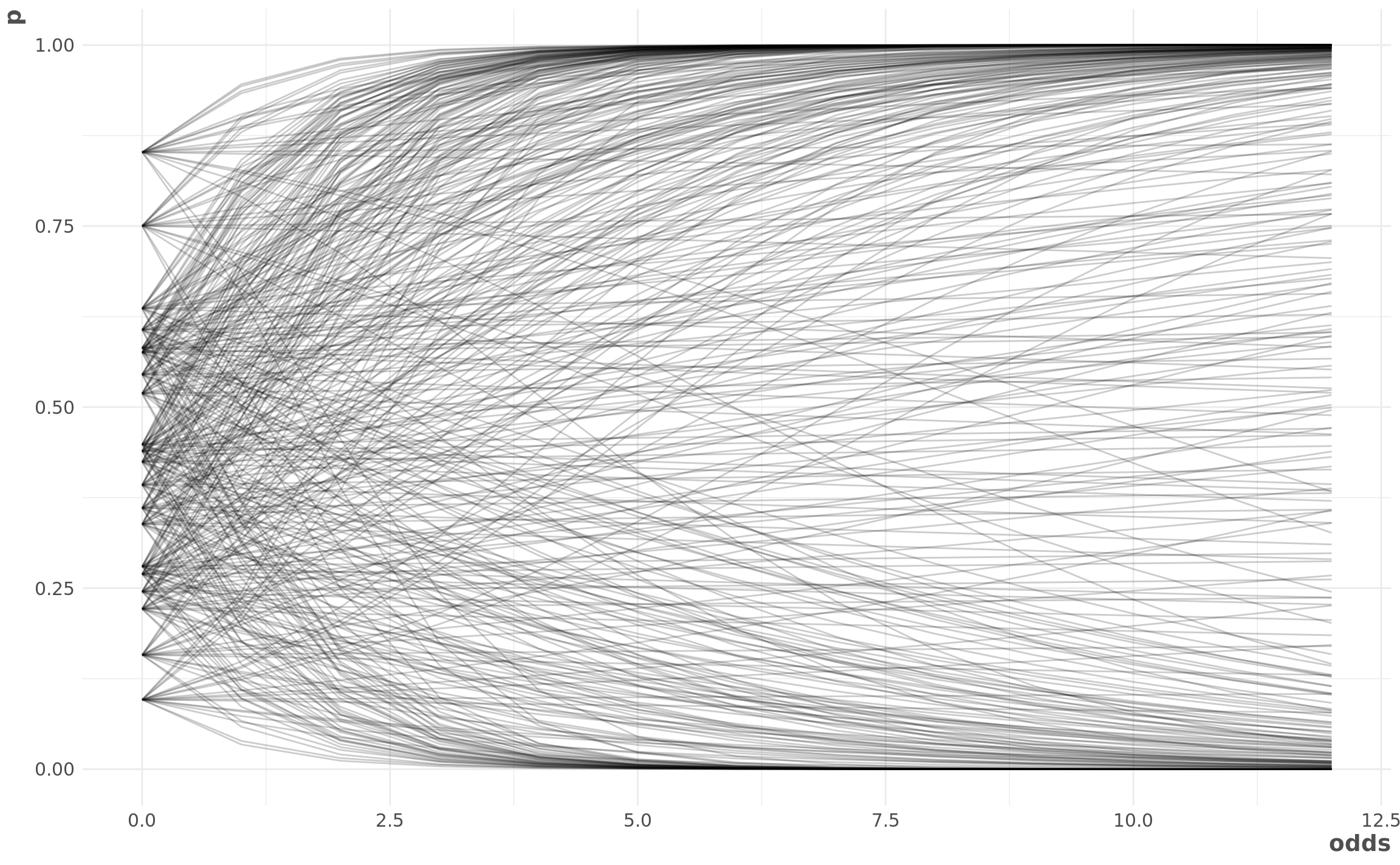
Looks ok to me!
Run the model
We’ll set-up our and run our model using the rethinking package as an interface to Stan.
set.seed(2020)

dat_list <- list(
    team = as.integer(as.factor(results_2019$team)),
    wins = results_2019$wins,
    n_games = 162L,
    log_odds = log(odds$odds[odds$year == 2019])
)

win_prob_model <- ulam(
    alist(
        wins ~ binomial(n_games, p),
        logit(p) <- a + b * log_odds,
        a ~ normal(0, 1),
        b ~ normal(0, 0.5)
    ),
    data = dat_list,
    chains = 4,
    iter = 2000,
    cores = parallel::detectCores()
)

precis(win_prob_model)
## mean sd 5.5% 94.5% n_eff Rhat4
## a 1.7592150 0.16142553 1.4906300 2.0136745 849.2970 1.000784
## b -0.2048753 0.01839704 -0.2341585 -0.1747385 855.5019 1.000390Posterior Predictive Checks
First, we’ll examine how this model performs on the data that we used to train it.
post_dat <- tibble(
    n_games = 162,
    log_odds = seq(6, 12, by = 0.1)
)

post <- sim(win_prob_model, data = post_dat) / 162
post_mean <- apply(post, 2, mean)
post_pi <- apply(post, 2, PI, prob = 0.95)

post_dat %>%
    mutate(post_mean = post_mean,
           post_high = post_pi[2, ],
           post_low = post_pi[1, ]) %>%
    ggplot(aes(log_odds, post_mean)) +
        geom_line() +
        geom_ribbon(aes(ymin = post_low, ymax = post_high),
                    alpha = 0.5) +
        geom_point(data = as_tibble(dat_list),
                   aes(y = wins / 162)) +
        scale_x_continuous(
            labels = function(x)
                paste0("+", comma(round(exp(x), 0)))
        ) +
        scale_y_continuous(labels = percent) +
        labs(y = "win percentage",
             title = "Comparing model predictions to actual results from 2019 season",
             subtitle = "shared area shows 90% interval of simulated outcomes",
             x = "preseason WS odds (log scale)")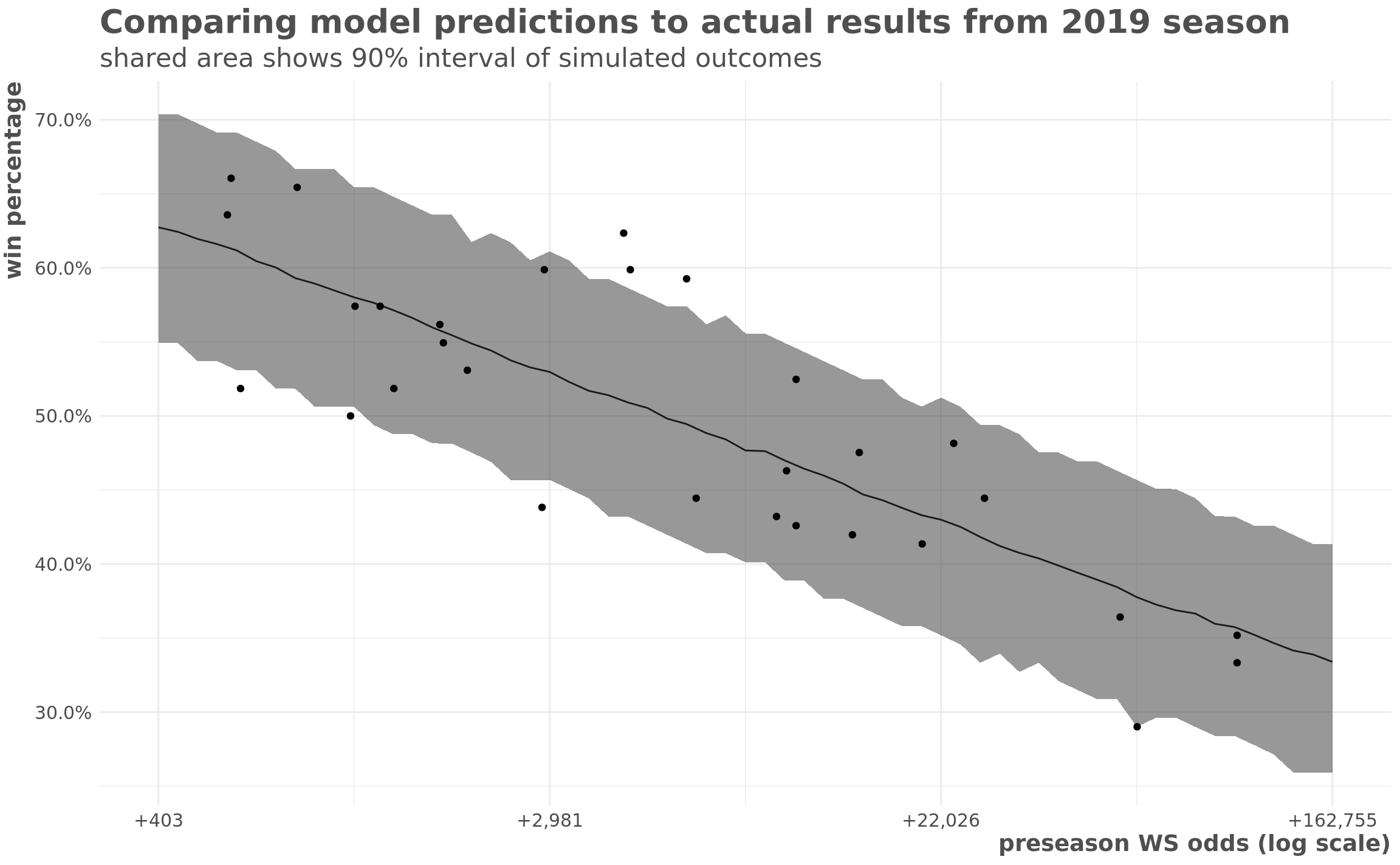
The model looks like it makes reasonable predictions. There’s a little bit more uncertainty in reality than the model predicts - the 90% interval has fewer than 90% of the teams’ actual records in it. But it looks pretty good.
How much uncertainty is there in this season?
What does it say about what we can expect this season? To figure this out, we’ll run simulated seasons from our model. The binomial distribution takes the form \({\sf Binom}(n, p)\) where \(n\) is the number of trials and \(p\) is the probability of success. We can run our simulations twice, once using \(n = 162\) for a full season and once using \(n = 60\) for the short season. Then we examine the distribution of percentages.
set.seed(2020)

pred_dat_short <- odds %>%
    filter(year == 2020) %>%
    mutate(log_odds = log(odds),
           n_games = 60)

pred_dat_full <- odds %>%
    filter(year == 2020) %>%
    mutate(log_odds = log(odds),
           n_games = 162)

preds_short <- sim(win_prob_model,
                   post = extract.samples(win_prob_model),
                   data = pred_dat_short)
pred_pi_short <- apply(preds_short, 2, PI)

preds_full <- sim(win_prob_model,
                   post = extract.samples(win_prob_model),
                   data = pred_dat_full)
pred_pi_full <- apply(preds_full, 2, PI)

pred_dat_short %>%
    mutate(high_short = pred_pi_short[2, ] / 60,
           low_short = pred_pi_short[1, ] / 60,
           high_full = pred_pi_full[2, ] / 162,
           low_full = pred_pi_full[1, ] / 162) %>%
    gather(type, val, high_short:low_full) %>%
    separate(type, into = c("int", "season")) %>%
    spread(int, val) %>%
    mutate(team = fct_reorder(team, high)) %>%
    ggplot(aes(team, color = season)) +
        geom_errorbar(aes(ymin = low, ymax = high),
                      size = 1, position = "dodge") +
        coord_flip() +
        scale_y_continuous(labels = scales::percent) +
        labs(y = "win percentage",
             x = "",
             color = "season length",
             title = "Range of win percentages wider in the short season",
             subtitle = "bars show 90% intervals of 4000 of 2020 season")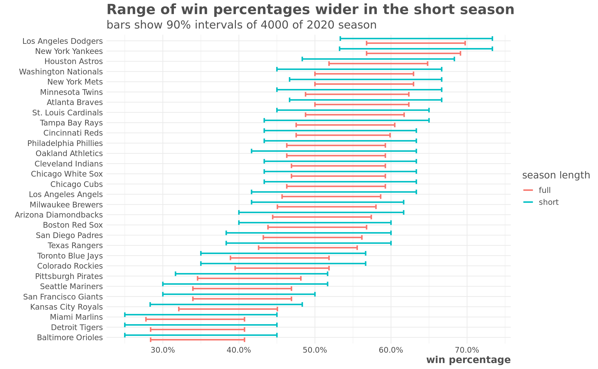
Clearly there is a much wider range of plausible outcomes for the short season. But those ranges look pretty wide in either scenario, and just looking at win percentage doesn’t really tell the whole story. Really we’re concerned with the variation in the possible final positions of each team within their division. So how does that change?
team_names <- results_2019 %>%
    mutate(team_num = as.integer(as.factor(results_2019$team))) %>%
    select(team_num, team, league)

count_outcomes <- function(preds, n_games) {
    preds %>%
    as.data.frame() %>%
    gather(team_num, wins) %>%
    mutate(
        n_games = n_games,
        pct = wins / n_games,
        team_num = as.integer(str_remove(team_num, "V")),
    ) %>%
    left_join(team_names, by = "team_num") %>%
    group_by(team) %>%
    mutate(sim = row_number()) %>%
    ungroup()

}

outcomes <- bind_rows(
    count_outcomes(preds_short, 60),
    count_outcomes(preds_full, 162)
)

outcomes_summary <- outcomes %>%
    group_by(sim, league, type = if_else(n_games == 60, "short", "full")) %>%
    arrange(desc(pct)) %>%
    mutate(position = row_number()) %>%
    ungroup() %>%
    group_by(team, league, type) %>%
    count(position) %>%
    mutate(pct = n / sum(n)) %>%
    ungroup()


outcomes_summary %>%
    mutate(team = fct_rev(fct_reorder2(team, position, pct, weighted.mean))) %>%
    ggplot(aes(position, pct, fill = type)) +
        geom_col(position = "dodge") +
        facet_wrap(league ~ team, ncol = 5) +
        scale_y_continuous(labels = percent) +
        labs(x = "division rank",
             y = "percent of simulations",
             title = "Final division position of different season outcomes",
             subtitle = "Based on 4000 simulations each of full and shortened seasons")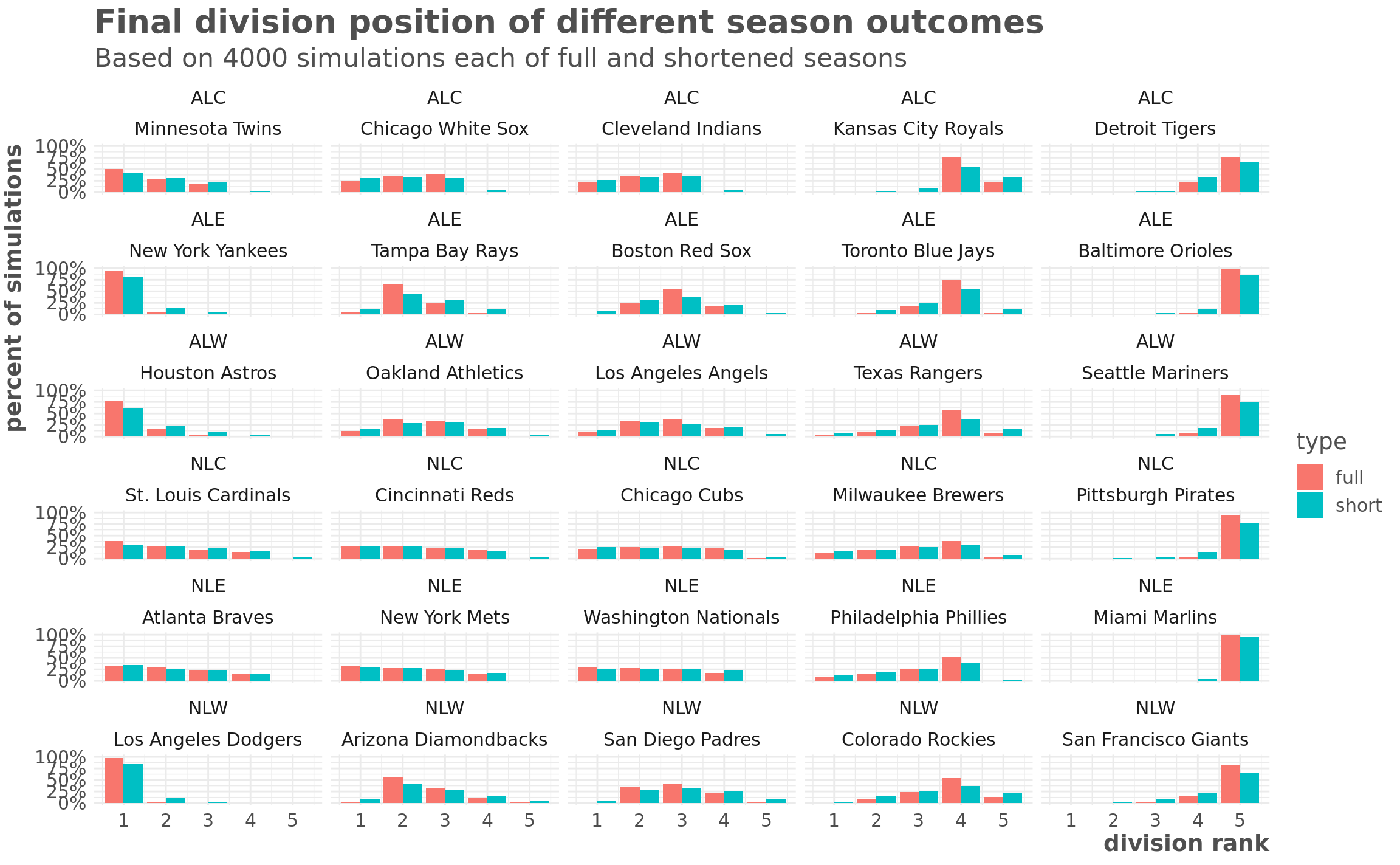
Some things really stand out here. First, at the extreme ranges, there isn’t actually that much variation. Its really unlikely the Yankees or Dodgers finish out of first, and its also really unlikely that the worst teams - Marlins and Orioles - will finish above last.
A lot of these divisions have a lot of potential outcomes regardless of whether it’s a short or long season. For example, this model predicts that the Cardinals or the Braves could finish first or fourth regardless of how long the season is.
Where things will potentially shake out in weird ways is in the middle of the pack. The table below shows the teams where the difference in the likelihood of a team finishing in a particular position between the shortened and a full season. The Blue Jays and the Royals both finish in fourth around 75% of time in the full season but just 55% of the time in the shortened season.
greatest_differences <- outcomes_summary %>%
    complete(team, position, type, fill = list(n = 0, pct = 0)) %>%
    group_by(team, position) %>%
    summarise(dif = pct[type == "full"] - pct[type == "short"]) %>%
    ungroup() %>%
    top_n(10, abs(dif))

outcomes_summary %>%
    semi_join(greatest_differences, by = c("team", "position")) %>%
    select(-n) %>%
    spread(type, pct)  %>%
    mutate(difference = round((full - short) * 100, 2)) %>%
    arrange(desc(abs(difference))) %>%
    mutate_at(vars(full, short), percent, 0.01) %>%
knitr::kable()| team | league | position | full | short | difference |
|---|---|---|---|---|---|
| Tampa Bay Rays | ALE | 2 | 66.62% | 45.02% | 21.60 |
| Toronto Blue Jays | ALE | 4 | 75.95% | 54.62% | 21.32 |
| Kansas City Royals | ALC | 4 | 76.55% | 55.97% | 20.57 |
| Texas Rangers | ALW | 4 | 56.57% | 38.55% | 18.02 |
| Boston Red Sox | ALE | 3 | 55.95% | 38.22% | 17.73 |
| Seattle Mariners | ALW | 5 | 91.00% | 73.68% | 17.33 |
| Colorado Rockies | NLW | 4 | 54.00% | 36.75% | 17.25 |
| San Francisco Giants | NLW | 5 | 81.55% | 64.32% | 17.23 |
| Pittsburgh Pirates | NLC | 5 | 94.82% | 78.00% | 16.83 |
| Houston Astros | ALW | 1 | 76.35% | 61.70% | 14.65 |
| New York Yankees | ALE | 1 | 94.68% | 80.02% | 14.65 |
Conclusion
The baseball season will potentially shake out in really interesting ways this year. Some of this is due to the shortened season, and some of this is due existing parity in baseball.
