
Does it rain more on Tuesdays (with informative priors)?
A couple of years ago, I wrote about rain on different days of the week in Philadelphia. I was annoyed because it felt like every time I took out the trash, it was raining. Our trash day is Wednesdays, so I take it out on Tuesday nights. When I did that analysis, I found that, sure enough, it did rain more on Tuesdays! Maybe not that interesting - it’s gotta rain more on some day, right? The surprising thing though was that the confidence interval for Tuesday did not include 0. So I could reject my null hypothesis that it rained the same amount on each day and say my results were statistically significant.
This article exemplifies a typical argument in the frequent vs Bayesian, even if the title - ‘Bayesian Estimation with Informative Priors is Indistinguishable from Data Falsification’ - is somewhat provocative. The argument goes that using priors is basically just manipulating the data to get the results you want. This puts Bayseians in something of a catch-22: if you use informative priors, you could be seen as fiddling your data to find the outcomes you want; if you use uninformative priors, then you’re just doing frequentist statistics!
Reading this recently made me think about the rain on Tuesdays article. At the time, my view was that this was a fluke of randomness; occasionally you will find a result that looks like there is something going on when there isn’t. Obviously the day of the week doesn’t impact the weather. I was really just joking when I did it the first time and didn’t expect to find anything. However, maybe a Bayesian approach will give us an answer that we know is more in line with reality.
library(tidyverse)
library(lubridate)
library(here)
library(rstanarm)
library(jtcr)
library(broom)
library(pROC)

theme_set(theme_jtc())


# use same data that goes up to September 2018
weather <- "https://jtcies.com/data/phl_weather_20090925-20180924.csv" %>%
  read_csv(guess_max = 2000) %>%
  janitor::clean_names()

weather_processed <- weather %>%
    mutate(
        dow = as.factor(wday(date)),
        rain = as.integer(prcp > 0)
    )
Below is the percentage of days that it rained in Philadelphia by day of the week:
weather_processed %>%
    group_by(`day ofweek` = dow) %>%
    summarise(
        n = n(),
        `percent rainy days` = mean(rain)
    ) %>%
knitr::kable()| day ofweek | n | percent rainy days |
|---|---|---|
| 1 | 469 | 0.2857143 |
| 2 | 469 | 0.3198294 |
| 3 | 469 | 0.3859275 |
| 4 | 469 | 0.3262260 |
| 5 | 469 | 0.3411514 |
| 6 | 470 | 0.3063830 |
| 7 | 469 | 0.3176972 |
Comparing Models
We’ll fit four models to see how the priors impact the coefficients. My assumption is that the day of the week has no impact on whether it rains so models that produce coefficients closer to zero should be closer to what we’d expect. The first model is a likelihood model and the next three are Bayesian models with increasingly informative priors.
mod1 <- glm(
    rain ~ dow,
    family = binomial(link = "logit"),
    data = weather_processed
)

mod2 <- stan_glm(
    rain ~ 1 + dow,
    family = binomial(link = "logit"),
    data = weather_processed,
    prior = normal(0, 0.5),
    prior_intercept = normal(-0.8, 1)
)

mod3 <- stan_glm(
    rain ~ 1 + dow,
    family = binomial(link = "logit"),
    data = weather_processed,
    prior = normal(0, 0.25),
    prior_intercept = normal(-0.8, 1)
)

mod4 <- stan_glm(
    rain ~ 1 + dow,
    family = binomial(link = "logit"),
    data = weather_processed,
    prior = normal(0, 0.1),
    prior_intercept = normal(-0.8, 1)
)
extract_coef <- function(x) {
labels <- c("Intercept", as.character(wday(2:7, label = TRUE)))
priors <- prior_summary(x)$prior
dist <- priors$dist
mu <- unique(priors$location)
sigma <- unique(priors$scale)
if (is.null(priors)) {
prior_label <- "no prior"
} else {
prior_label <- paste0(dist, "(", mu, ", ", sigma, ")")
}
tidy(x) %>%
mutate(param = labels,
prior = prior_label)
}
results <- list(mod1, mod2, mod3, mod4) %>%
map_dfr(extract_coef, .id = "model")
results %>%
mutate(param = fct_rev(fct_inorder(param)),
prior = fct_rev(fct_inorder(prior))) %>%
ggplot(aes(param, estimate, color = prior)) +
geom_point(
size = 2,
position = position_dodge(width = 0.5)
) +
geom_linerange(
aes(ymin = estimate - 1.96 * std.error,
ymax = estimate + 1.96 * std.error),
position = position_dodge(width = 0.5)
) +
coord_flip() +
color_jtc("color") +
guides(color = guide_legend(reverse = TRUE)) +
labs(
title = "Informative priors get us closer to what we expect",
subtitle = "bars represent 95% interval around estimates",
y = "coefficient",
x = "parameter"
)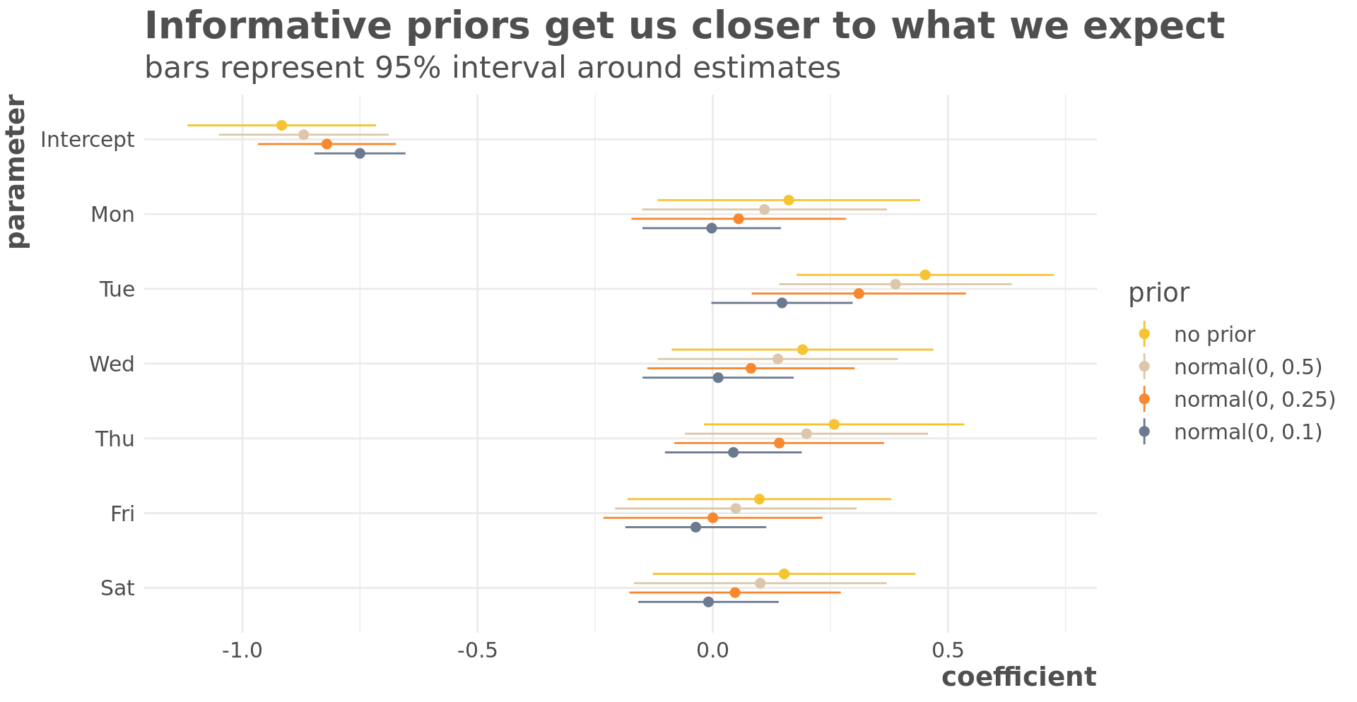
The more informative our priors, the closer they get us to our expectation that day of the week has no impact on rain.
The informative priors don’t substantially change the predictions in this example. There are very slight differences with more informative priors having a negative impact on in-sample fit and a better impact on out-of-sample fit.
calc_roc <- function(x) {
    preds <- augment(x, type.predict = "response")

    area_under <- auc(roc(preds, rain, .fitted,
                          direction = "<",
                          levels = c(0, 1)))

    threshold <- seq(0, 1, by = 0.01)

    pred_levels <- preds %>%
        nest(data = everything()) %>%
        crossing(threshold) %>%
        unnest(data) %>%
        mutate(
            tp = .fitted >= threshold & rain == 1,
            fp = .fitted > threshold & rain == 0
        )

    pred_levels %>%
        group_by(threshold) %>%
        summarise(
            tpr = sum(tp) / sum(rain == 1),
            fpr = sum(fp) / sum(rain == 0)
        ) %>%
        mutate(area_under = as.numeric(area_under))
}

list(mod1, mod2, mod3, mod4) %>%
    map_dfr(calc_roc, .id = "model") %>%
    left_join(
        results %>%
            distinct(model, prior),
        by = "model"
    ) %>%
    mutate(
        prior = paste0(prior, " | AUC: ", round(area_under, 3)),
        prior = fct_rev(fct_inorder(prior))
    ) %>%
    ggplot(aes(fpr, tpr, color = prior)) +
        geom_line(size = 2, alpha = 0.5) +
        expand_limits(y = c(0, 1), x = c(0, 1)) +
        color_jtc("color") +
        guides(color = guide_legend(reverse = TRUE)) +
        labs(title = "Most informative priors perform worst on in-sample predictions",
             x = "False positive rate",
             y = "True positive rate")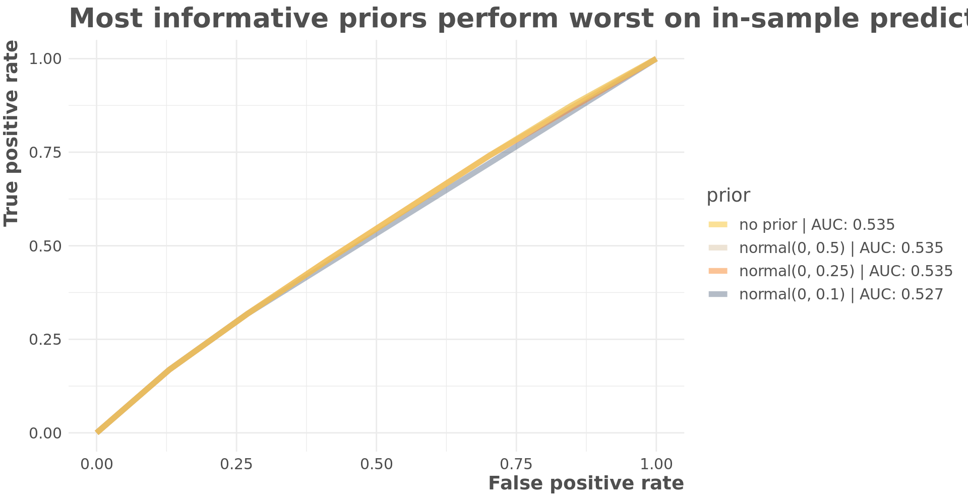
Informative priors perform best on out of sample predictions.
loo_compare(loo(mod2), loo(mod3), loo(mod4)) %>%
knitr::kable()| elpd_diff | se_diff | elpd_loo | se_elpd_loo | p_loo | se_p_loo | looic | se_looic | |
|---|---|---|---|---|---|---|---|---|
| mod4 | 0.0000000 | 0.000000 | -2073.585 | 19.56417 | 3.777437 | 0.0519723 | 4147.171 | 39.12835 |
| mod3 | -0.2747685 | 1.275200 | -2073.860 | 19.71171 | 6.001727 | 0.0798861 | 4147.721 | 39.42341 |
| mod2 | -0.3594907 | 1.841144 | -2073.945 | 19.75817 | 6.569758 | 0.0864072 | 4147.890 | 39.51634 |
Conclusion
I wanted to revisit this because the original analysis always felt strange to me. I was right that it did rain more on Tuesdays, and this gave my wife and I something to joke about. But day of the week doesn’t actually do anything to the weather, but you could interpret my results to say that it did (within some probability).
As discussed in the article I referenced above, the frequentist analysis asks “What’s the probability of the data given the hypothesis that day of the week has no impact on whether it rains.” We saw that there was a pretty small chance of that. The Bayesian analysis asks “What’s the probability that day of week has some impact on whether it rains given the data?” There’s still some chance it does but we’re less sure.
It seems to me that the technique should be based on the question you want answered and the data you have. In this case, using informative priors gave me something closer to what I’d expect.
